Chembricks Blog
A head start from physics beats a bigger AI model
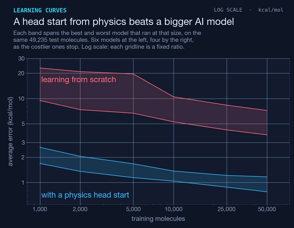
There are two ways to make an AI model better at chemistry. You can make the model bigger and feed it more data. Or you can give it a head start, by having it correct a fast, rough physics calculation rather than work everything out from nothing.
We tested both, with six machine-learning models. Two are ours, chembricks-phy-AI-1 and chembricks-phy-AI-2. The other four are well-known models from the literature. They range from a compact kernel method, which works quite differently from a neural network, to some of the best-known neural networks in chemistry, all predicting the same property of the same molecules, all scored on the same 49,235 molecules that none of them ever trained on. One of the six, chemprop, reads only the flat structure diagram while the others get the 3-D geometry, which is worth remembering wherever it appears below. We also measured exactly how much computing time each one burned.
The head start won, and it was not close.
What the models were asked to do
The task is to predict a molecule's energy. Energy sounds abstract, but it is the quantity underneath most of the questions chemists actually ask. Which of these two forms is the stable one? Will this reaction release heat or need it? Is this structure a real molecule or a drawing that would fall apart in a flask?
The reliable way to get that number is a quantum chemistry calculation. It is accurate and it is slow, which is why people want models that can approximate it in milliseconds.
So we gave the six models the same reference calculations to learn from, and set the task up two ways.
- From scratch. The model sees the molecule and predicts the energy. Nothing else goes in.
- With a head start. A fast approximate physics method called g-xTB takes a first guess, and the model only has to learn the difference between that guess and the truth.
The second setup asks much less of the model. It never has to learn the bulk of the physics, because the physics has already been done. It only has to learn where the quick calculation goes wrong.
Errors below are averages of the absolute error, in kcal/mol. For scale, chemists traditionally call 1 kcal/mol chemical accuracy, meaning good enough to trust for real decisions. The rough physics guess on its own, with no model correcting it, sits at about 2.9.
The head start matters more than the model you pick
In the figure above, the two bands hold the same six models. The only difference is whether the physics ran first. The gap between the bands is larger than the spread of models inside either one.
The sharpest way to put it: the worst result from any model with the head start, trained on just 1,000 molecules, is still better than the best result from any model without it, at any training size we ran, including runs on a thousand times more data. The figure stops at 50,000 molecules, where all but one model stopped; the larger runs are in the full tables.
That is worth sitting with. A great deal of effort in AI for science goes into larger models and larger datasets. Here, one cheap physics calculation was worth more than every architectural difference on the board combined.
What it costs is the striking part
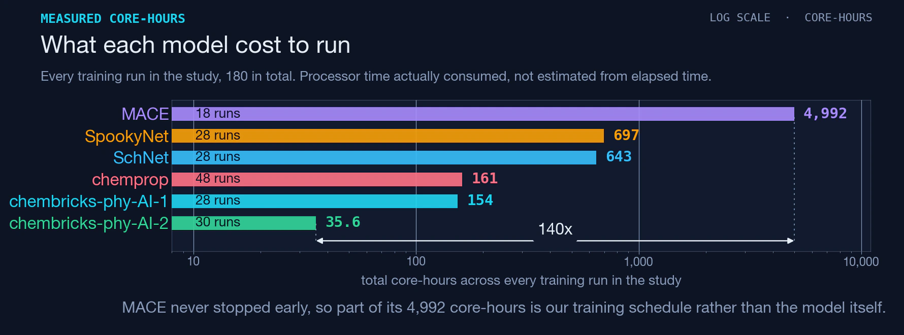
The most expensive model in the study, MACE, used 4,992 core-hours. The cheapest, our own kernel method chembricks-phy-AI-2, used 35.6. That is a factor of 140. One thing tempers it: MACE ran at its own default settings and never stopped training early, so part of that total is our schedule rather than the model.
Put the other way round: every run our model contributed to this study, thirty of them, across both setups and every training size, together cost about a quarter of what one single MACE training run cost at the smallest training size on the board.
And the expensive model did not buy accuracy with it. At every training size where both of them ran, on both setups, the cheap one was more accurate.
At the small end the numbers stop sounding like machine learning at all. With the physics head start, our model trained on 1,000 molecules in about three minutes of a single processor core, and landed at 1.682. No model in the study, at any training size, at any cost, got below 3.690 without that head start.
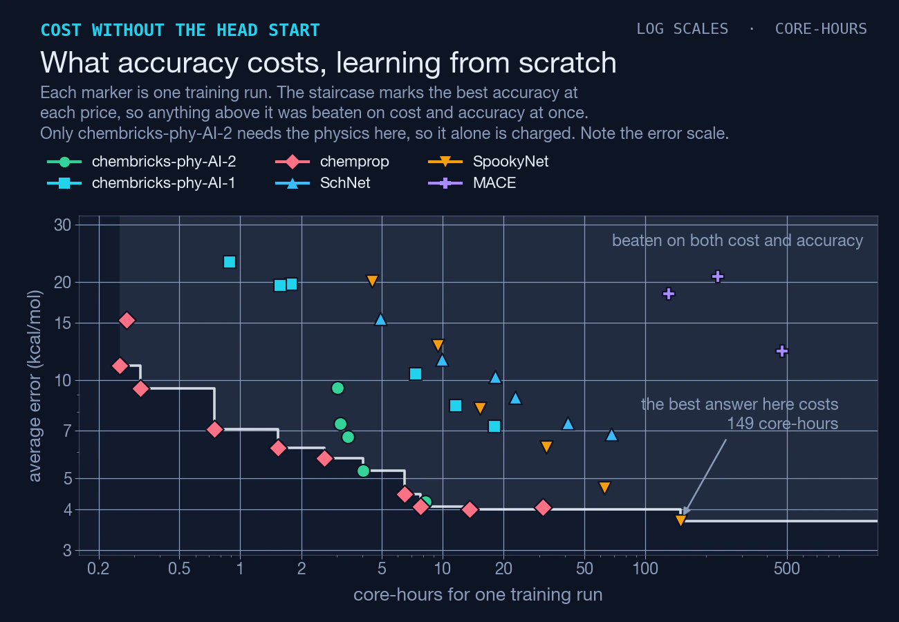
Plotting accuracy against cost makes the pattern easier to see. There is one plot per setup below, drawn the same way. The staircase marks the best accuracy available at each price, and anything above it is a run that something else beat on both counts at once.
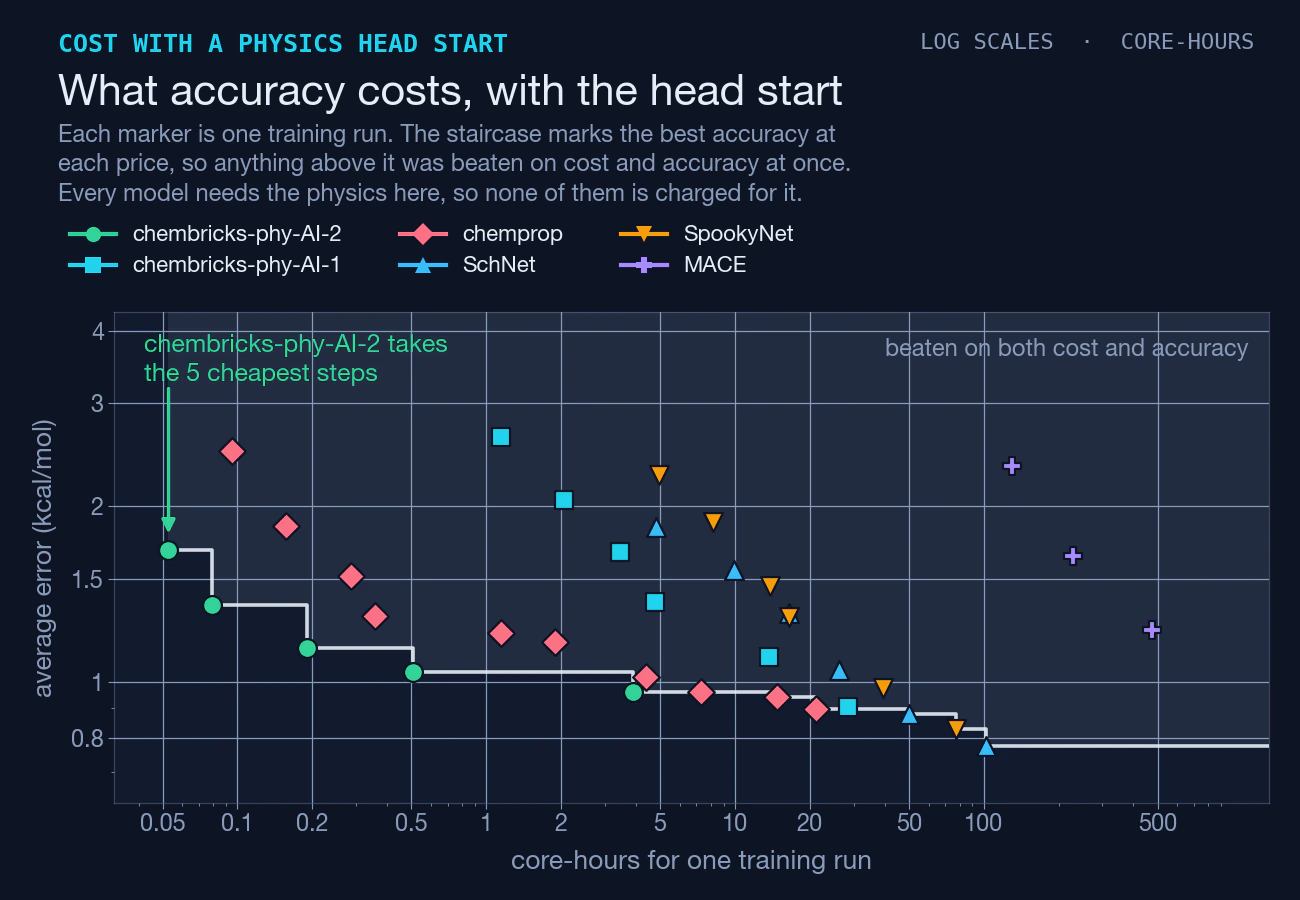
With the head start, the five cheapest steps of that staircase all belong to our model. It reaches an average error of 0.961 from 25,000 molecules, in under four core-hours of training.
Everything that beats it, beats it by paying. chemprop gets to 0.897, but it needs all 993,112 training molecules and five times the compute. SpookyNet gets to 0.829 for twenty times the compute. SchNet, the most accurate model in the study, needs twenty-six times the compute to cut the error by about a fifth. That is the trade on offer, and for most work it is not an attractive one.
Without the head start the same plot is a different shape. Every error is several times larger, chemprop holds most of the cheap end, and the best answer on the board costs 149 core-hours to train.
Where the big neural networks won
Two of the standout results here are not ours, and they deserve saying plainly.
SpookyNet was the most accurate model without any head start. Trained on 50,000 molecules it reached 3.690, while chemprop, trained on all 993,112, finished at 4.060, and its best anywhere was 4.000. Roughly twenty times less data, and a better answer. That is the largest data-efficiency result in the study, though it did not come cheaply: the run that produced it cost about five times the compute of chemprop's full-dataset run.
SchNet was the most accurate model with the head start, at 0.775, with SpookyNet behind it at 0.829. The kernel method that owns the cheap end lands at 0.961.
So the honest summary is not that our model is the most accurate. It is that it gets close to the best answer on the board for one or two orders of magnitude less compute to train. Where the physics head start is available, it matters more than which model you pick, and what you save is enormous.
A result we did not expect
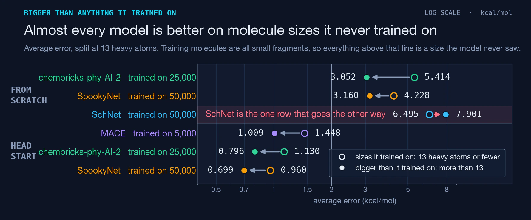
The training molecules are all small fragments. You would expect the models to do worse on molecules bigger than anything they had seen. We checked six model and size combinations spanning both setups, and five of them went the other way.
chembricks-phy-AI-2, learning from scratch on 25,000 molecules, averaged 5.414 on the small molecules and 3.052 on the large ones. SchNet learning from scratch was the one that behaved as expected.
We have a guess about why, and we are flagging it as a guess. The property being predicted depends heavily on which bonds are present, and a larger molecule contains more repeats of patterns the model has already seen, so its errors may average out. We have not shown that this is the reason.
The model you can use today
The approach that holds the cheap end of this study, a fast physics calculation with a learned correction on top, is the one behind a model already available in the Chembricks AI API and MCP server.
tool:     cmbx_organic_electronic_v2dl
endpoint: organic-electronic-wb97mv-v2dl
input:    a SMILES string, or a 3-D structure
returns:  total energy, HOMO, LUMO, HOMO-LUMO gap
One boundary worth stating: this study measured total energy only. The deployed model also returns orbital energies, and those are not covered by any number on this page.
A slice of the underlying data is public and free for anyone, under an MIT license: chembricks/WB96MV-ORGANIC on Hugging Face, 801,781 molecular structures with reference energies, orbital energies and full provenance.
The full numbers
Every table behind these figures, all 72 accuracy-against-cost points, the exact protocol, how the test set was built and the methodological detail left out above, are on the complete results page. The figures here and the tables there are generated from one committed data file, so they cannot drift apart.
Access is open to anyone. You can call the model discussed here, and the rest of the physics validation layer, from Chembricks AI.
Get new articles by email
Notes on physics validation for AI chemistry, straight from the team. No spam.
Double opt-in. Unsubscribe anytime.